Module 6 - Working with Geometries

In the final module of this course, Module 6, we will explore the topic of geometries. This includes learning how to interpret the properties of geometry objects derived from existing features, as well as the process of creating new geometry objects based on coordinate information.

Features are objects that are depicted on a map or within a dataset. A point represents a single location like a fire hydrant or a tree; a polyline represents a linear feature such as a road, river, and a polygon feature that represents an area or region, like a lake, park, or administrative boundary. Each feature in a data set is typically represented by a row in an attribute table.

A point feature class in GIS represents a single location consists of a single vertex defined by x,y coordinates. On the other hand, polyline and polygons features consist of multiple vertices and are constructed using two or more points objects. These vertices define the shape of a polyline or polygon feature.

To effectively work with geometry objects, it is essential to establish a cursor on the geometry field. Tokens such as SHAPE@ provide access to the complete geometry object; however, in the context of a large dataset, this approach may lead to slower performance. For scenarios where only specific properties are required, alternative tokens can be utilized. For instance, SHAPE@XY returns a tuple of x and y coordinates that represent the centroid of the feature, while SHAPE@LENGTH provides the length of the feature.

ArcPy provides a variety of classes designed for working with geometry objects, including the generic arcpy.Geometry class, which is utilized to create geometry objects. In addition to this, ArcPy includes four specific geometry classes: MultiPoint, PointGeometry, Polygon, and Polyline. Furthermore, ArcPy incorporates two additional classes that facilitate the construction of geometry: Array and Point. The relevant classes include arcpy.Array() and arcpy.Point().

Certain features are composed of multiple parts but are represented as a single feature within the attribute table; these are referred to as multipart features. To determine whether a feature is classified as a single part or multipart, the isMultipart statement is utilized. Additionally, the partCount function will provide the total number of geometry parts associated with a given feature. Furthermore, polygons that contain holes present a challenge. These shapes typically feature one exterior ring, which is defined as a clockwise ring, and one or more interior rings that are defined as a counterclockwise ring.

Lastly, we explored the process of writing geometries, which encompasses the creation of new features. New features can be developed utilizing the InsertCursor class from the arcpy.da module. This process requires creating a geometry object, and then saving the result as a feature using insertRow() method.

cursor = arcpy.da.InsertCursor()

The lab assignment for Module 6 requires the development of a Python script that generates a new text file. This script should populate the file with the Object Identifier (OID) of each feature or row, the vertex ID, the X and Y coordinates of the vertices, as well as the name of the river feature derived from a feature class containing polylines representing rivers in Maui, Hawaii.

Initially, I imported all necessary modules and classes, enabled the overwriteOutput setting, configured the workspace, and defined the feature class variable. Subsequently, I created a rivers.txt file in write mode ("w") and established a search cursor for the rivers.shp file. This cursor was designed to access the OID, SHAPE, and NAME fields.

Furthermore, I implemented a for loop to iterate through each row or feature within the cursor/ShapeFile, while also creating a variable to serve as a vertex ID number. A second for loop was introduced to iterate through each point or vertex in the row, utilizing the .getPart() method to extract the x and y coordinates of the vertices, incrementing the vertex ID number with each iteration.

The output.write() method was employed to append a line to the .txt file, detailing the Feature/ROW OID, Vertex ID, X coordinate, Y coordinate, and the name of the river feature. A print statement was also included to display the output.write result. Finally, I ensured that the .txt file was properly closed and deleting row and cursor variables outside of all loops.

The execution of the script for Module 6 generated a formatted text file corresponding to each river feature within the Maui rivers feature class.

 

Module 6 script flowchart

Module 5 - Exploring & Manipulating Data

This module provides an in-depth examination of methods for exploring spatial data, including checking for datasets, describing, and listing data in a workspace. Additionally, it addresses the utilization of lists, tuples, and dictionaries, as well as the application of for loops in lists. For loops are fundamental tools in Python for working with lists and other iterable objects. They allow you to execute a block of code repeatedly, once for each item in the list.

In the second segment of the module, which focuses on data manipulation, we are introduced to the use of cursors for data access, the integration of SQL within Python, and the management of table and field names. The module places a strong emphasis on the use of cursors to traverse table rows, highlighting various types for executing search operations, adding new records, and updating existing ones. Furthermore, it covers the essential topic of validating text and field names to ensure data integrity.

In this lab, we will develop a script composed of three code blocks. The initial block is designed to establish a new file geodatabase (fGDB) and transfer existing shapefiles from the Data folder into the newly created geodatabase. The second block involves creating a Search Cursor to extract and display the city NAME, FEATURE, and POP_2000 fields for cities identified as 'County Seats'. Lastly, we will initialize an empty dictionary and fill it with the names (as keys) and populations (as values) of all County Seat cities and utilizing a for loop to print the dictionary.

After importing the necessary modules and classes, and setting overwriteOutput to True, we created an empty geodatabase in the Module5/Results folder using the arcpy.CreateFileGDB_management statement. Next, we defined the fclist variable to enumerate all feature classes in the current workspace, followed by creating a for loop to transfer all features from the Data folder to the new geodatabase (fGDB).

When transferring shapefiles to a file geodatabase (fGDB), it is essential to modify the names appropriately. The default naming convention for shapefiles includes the file extension “.shp,” which must be removed. it necessary to use the Describe() functions basename property of shapefiles when copied via Python script from a folder to a file geodatabase. The script utilizes the basename property of the feature class instead of the default name for the feature class that is stored within the fGDB.

The subsequent section of the script involves establishing a Search Cursor for the cities layer to retrieve the Name, Population (POP_2000), and Feature of all cities designated as 'County Seat' in the Feature field. To achieve this objective, we must first configure the workspace to the new fGDB workspace. Once the variables are set and the Delimited field is established, we created a Search Cursor. We then utilize a for loop within the cursor to display all the cities' NAME, POP_2000, and FEATURE categorized as 'County Seat.'

The last block of code in the script is to create an empty dictionary and populate it with names (keys) and populations (values) of each 'County Seat' city, and print the populated dictionary using a for loop. This final step of the lab assignment presented significant challenges for me. I successfully created the empty dictionary and implemented the for loop utilizing the format <dictionary variable>.update({<key>:<value>}). However, upon execution, I did not encounter any error messages, yet the output was not as anticipated. I reviewed the materials from Module 5, including exercises and lectures, and conducted further research online, but I was unable to identify the error. I discovered that the print statement had incorrect indentation; after correcting the indentation and rerunning the script, the script ran successfully and the output met my expectations.

Here is a screen shot showing the output of the Module 5 Python script       

              

Module 5 Python script flowchart

Module 4 - Geoprocessing

This week’s module covered geoprocessing with Python using the ArcPy package. ArcPy is a collection of modules as well as functions and classes that enhance Python's capabilities. To start working with ArcPy we first need to import the package by using the line of code import arcpy. Once arcpy is imported all geoprocessing tools found in ArcGIS Pro can be run.

The subsequent step involves configuring the workspace to the default location designated for the input and output files that will be utilized in our tasks. This can be accomplished by employing the arcpy.env.workspace function. The syntax to be followed is arcpy.<class>.<property>, where 'env' is classified as a class, and 'workspace' serves as a property of this class.

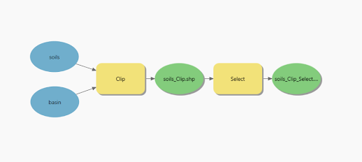
Module 4 exercise focused on geoprocessing with ArcGIS Pro, we utilized the Clip tool from the analysis toolbox to clip the soils shapefile with the basin shapefile. Subsequently, we performed a batch process using the Clip tool to clip multiple shapefiles, including flood zones, lakes, rivers, and roads. Additionally, this exercise provided us with the opportunity to learn how to configure geoprocessing options and to explore models and the ModelBuilder feature in ArcGIS Pro.

In the lab assignment, we undertook two primary tasks. The first task involved the creation of a model designed to identify all soils within the basin shapefile feature that are currently or potentially suitable for agricultural purposes. The second task required the development of a script to execute three geoprocessing functions utilizing ArcPy.

To initiate the first task, we ensured that the option to "Allow geoprocessing tools to overwrite existing datasets" was enabled. This setting can be configured via the options menu under geoprocessing. We then created a new project and incorporated the shapefiles for soils and basin into a new map. Subsequently, we established a new toolbox and a new model named "SoilErase." Locating the Clip tool within the geoprocessing analysis toolbox and adding it to the model. Double-clicking on the Clip tool, to accessed the tool dialog box, where we designated "soils" as the input features and "basin" as the clip features. Upon executing the model, a new shapefile, "Soils_Clip," was generated and saved in the default directory, and added to the project.

Clip tool

The next phase involved selecting all soils classified as "Not prime farmland" for removal from the shapefile. To achieve this, we incorporated the select tool from the geoprocessing toolbox. After double-clicking the select tool, we designated "Soils_Clip" as the input feature. To eliminate soils classified as "Not prime farmland," we added the expression [FARMLNDCL] <> 'Not prime farmland' to select all entries that do not fall under this classification within the [FARMLNDCL] field of the attribute table. Running the model the new shape file “Soil_Clip_Select is being created and added to the project.

 

Selection tool

Created Clip_Select Model 

Screenshot of the final result

The second task required the development of a script to execute three geoprocessing functions utilizing ArcPy. There are various approaches to complete this task effectively. Initially, I duplicated the existing shapefile from the Data folder to the Result folder. This practice guarantees that the original layer remains untouched and serves as a backup. Subsequently, I incorporated the XY coordinates into the new shapefile. Following this, I proceeded to create a buffer and, ultimately, performed a dissolve operation. Although the Buffer and Dissolve processes can be executed in a single statement, I chose to implement them as two distinct statements. This decision allows for the generation of two separate layers for the buffer: one containing all individual buffers and the other representing the dissolved buffer.

1. First, I Imported arcpy, and from arcpy import env to set the workspace to the Data folder.

2. In order to enable the script to overwrite outputs, it is essential to check the option “Allow

geoprocessing tools to overwrite existing datasets” within the Geoprocessing settings in ArcGIS Pro

options. Additionally, to ensure that outputs can be overwritten during geoprocessing operations in Python IDLE, it is necessary to include the command “arcpy.env.overwriteOutput = True.”

3. Using arcpy.Copy_management to copy the shape file from the Data folder to the Results folder.

4. Using env.workspace to change and reset the workspace to the Results folder where the new shapefile is been saved.

5. Using arcpy.AddXY_management to add XY coordinates to the new copied shapefile.

6. Using the arcpy.Buffer_analysis and consequently arcpy.Dissolve_management to create a 1000 meter around the hospital features and then dissolve the created buffers into a single feature. The dissolve buffer step can be combined with the Buffer statement by using ALL in the buffer statement.

Using ALL for the dissolve_option instead of NONE will dissolve all buffers together into a single feature, removing any overlap.

arcpy.analysis.Buffer(in_features, out_feature_class, buffer_distance_or_field, {line_side}, {line_end_type}, {dissolve_option}, {dissolve_field}, {method})

7. Adding a print statement at the beginning of each task block and GetMassages() function at the end. This modification will ensure that when the script is executed, it displays an explanation of the processes being carried out, along with the respective start and end times.

Running the code from Notebook ArcGIS Pro 

Running the code in Python IDLE 

Flowchart for Module 4 lab

 

 

 

 

 

Module 3 - Debugging and Error Handling

This week's module focuses on debugging procedures and provides a comprehensive review of the most prevalent errors encountered in Python programming. We have explored syntax errors and exceptions, established a shortcut to the Integrated Development and Learning Environment (IDLE), debugged a script within IDLE, and learned how to handle exceptions using the try-except statement. 

Additionally, we have been introduced to the built-in syntax checking feature in Python IDLE, which allows for a syntax verification without executing the code through the interpreter. A pop-up dialog box will appear to notify users of any syntax errors detected. It is important to note that while the error check indicates the location of the syntax error, it does not specify the exact nature of the error, such as whether a colon is missing.

Syntax errors arise when the code does not adhere to the established rules of the Python programming language. Common causes of these errors include misspelled keywords, incorrect punctuation, omitted colons, and errors in indentation. Conversely, run-time errors, also known as Exception errors, occur when the interpreter encounters a situation that it cannot process. If these exceptions are not managed appropriately, the script will terminate unexpectedly. 

The laboratory exercise focused on debugging and error handling and was divided into three parts. 

Part 1 involved a script containing two errors. After executing the script, I was able to identify and rectify the errors, resulting in a successful execution of the script. The intended outcome of the script was to print the names of all the fields in the parks shapefile.

Module 3 – Part 1 results 

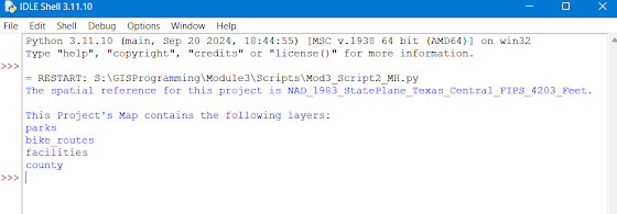
The second part of the lab assignment focused on identifying and rectifying additional errors and exceptions. Prior to executing the script, we ensured that the four shapefiles were incorporated into the project file named TravisCountyAustinTX.apx. The expected result upon successful execution of the script is the display of the names of all layers within the project.

Module 3 – Part 2 results

Part three of the lab assignment was about using the try-except statement to make a code run even with errors. The try-except statement in Python is used for handling exceptions errors. This functionality enables us to evaluate a block of code for potential errors and manage those errors effectively, thereby preventing the program from encountering a crash. The try-except statement traps the exception and provide additional error handling. 

Process of adding the try-except statement to the script:

1. Running the code, the first time resulted in receiving an error message line 13 

project = arcpy.mp.ArcGISProject() TypeError: ArcGISProject.__init__() missing 1 required positional argument: 'aprx_path' 

This error indicates that when we are trying to create an instance of the ArcGISProject class, we are not providing the necessary aprx_path argument.

2. To verify arguments and to catch any exception I added try-except statement. Prior to proceeding with this task, I verified that the file exists and confirmed that both the name and location are accurate

Try: placed before the first argument where the error exists and except Exception at the end of part A. Assigning a variable e and a print command

except Exception as e:

        print (e)

3. Executed the program once more, resulting in an error message for part A while part B executed successfully, displaying the name, data source, and spatial reference for each layer.

Module 3 - Part 3 results

Flowchart Part 3: Making a code run even with errors using try-except statement

Logic errors in Python, or semantic errors, arise when code executes without crashing but yields unintended or incorrect results due to a misalignment between the program's logic and the programmer's intended outcome. Unlike syntax errors, which halt execution, or runtime errors, which occur during operation, logic errors can be more difficult to detect.

Debugging is the process of identifying and removing errors from a program. Python offers several ways to debug code, which include:

1. Carefully reviewing the content of error messages.

2. Adding print messages to the script: Adding print messages after each geoprocessing tool or other important steps to confirm they were run successfully.

3. Selectively commenting out code: Involve removing certain lines to see if this eliminates the error. Double number signs (##) can be used to manually comment out lines of code.

4. Using Python debugger: A debugger is a tool that allows us to step through the code line by line, to place breakpoints in the code to examine the conditions at that point, and to follow how certain variables change throughout the code.

        a. Python built-in debugger called pdb

        b. IDLE debugger.

 

Module 2 - Python Fundamentals

During the second week of the GIS programming module, specifically in Exercise 2, we focused on the foundational elements of the Python programming language. This included working with various data types such as numbers, strings, variables, and lists. We explored the use of functions, methods, and modules, and learned how to save our code as scripts. Additionally, we practiced writing conditional statements and employing loop structures.

Furthermore, we gained practical experience in executing a geoprocessing tool from the notebook that interacts with a layer in ArcGIS Pro. We also learned the process of incorporating existing code into the ArcGIS Pro Notebook by copying and pasting the code into a notebook cell.

This week’s lab assignment comprises four distinct steps.

In the first step, the task involves assigning my full name as a string to a variable. Subsequently, the full name should be split into individual components, resulting in a list of names. Finally, indexing techniques will be employed to extract and print my last name.

The second step involves working with a prewritten code that generates a list of players participating in the dice game. Upon importing the random module and executing the code, I encountered an initial error TypeError: can only concatenate str (not "int") to str. To fix this error I added str to word (dice). After rectifying this issue and running the code again, I identified a second error, which required changing a capital 'X' to a lowercase 'x'. After addressing these errors, the code executed successfully.

In the third step, a loop must be created to generate and add 20 random numbers, each ranging from zero to ten, into a list. Finally, the fourth step requires the implementation of a loop designed to remove a specified integer from the previously generated list and print the updated list. 

Results from running the code:

In conclusion, completing the Lab for module 2 proved to be quite challenging, utilizing IDLE to compile the code in a separate script window was more efficient compared to ArcGIS Notebook and its cell functionality

Module 1 - Python Environments & Flowcharts

During the first week of GIS programming, we focused on executing Python scripts and engaging with the Python interpreter IDLE as well as Python (Jupyter) ArcGIS Notebook. Additionally, we examined flowcharts and developed our ability to think algorithmically through their use. 

Python is recognized as a simple yet powerful programming language. It is notably easier to learn compared to other programming languages, such as C++. Furthermore, it is free and open-source software. A key distinction of Python in relation to other programming languages is that it is an interpreted language. Unlike compiled languages, which necessitate a compiler to convert source code into machine code for execution, Python processes code sequentially, executing it line by line without the need for a compiler. This method of direct execution promotes a more straightforward approach to both code development and debugging. 

We were also introduced to various script editors and IDEs (Integrated Development Environments) that are utilized for writing and executing scripts. The three primary IDEs we explored for coding and testing purposes are IDLE (Integrated Development and Learning Environment), PyCharm, and Spyder. 

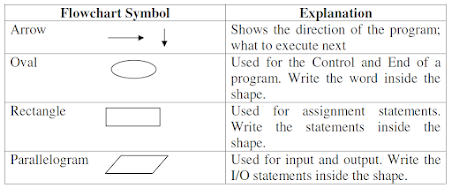
The second part of the module concentrated on flowcharts and their significance in programming, as they assist in visually and logically organizing a program. Flowcharts employ predefined symbols, such as ovals, rectangles, and parallelograms, to create a visual representation of the program. Arrows are utilized to indicate the direction of the program flow and the sequence of execution.

Agarwal_et_al_2010_Chapter 3 Page10

Utilizing our understanding of algorithmic thinking through flowcharts, we developed a flowchart to represent a Python script that converts 3 radians into degrees using the formula: Degrees = Radians * 180/Pi where Pi = 22/7 

Finally, this week, we were assigned to read "The Zen of Python" poem and to compose a paragraph reflecting our interpretation of its meaning.

“Zen of Python”, by Tim Peters, delves into the constitution of a well-established lines of code. In the poem, Tim remarks that a code must be well-structured or “beautiful”, as well as it directly and explicitly states what it does. A well-made code is simple; but if it were to be complex, it should not be made difficult. Tim remarks that a flat code, rather than nested, is better as it would be easily understood and more easily maintained. Furthermore, making a code neat and unscattered produces easy readability to its viewer.

According to the poet, even though there may be special cases, these special cases should never warrant a need to break the abovementioned rules. The poet goes on to say as well that although a practical code, as in one that works, may have a few errors, for instance, is better than a pure, mistake-free code, errors must never be left unlooked and remain unresolved. Furthermore, these errors must be found and fixed as soon as possible. Thus, a coder must always look for and research the best approach to building lines of code and refuse the urge to guess their work. The poet refers to Dutch programmer Guido van Rossum, the author of Python, stating that there is always one obvious approach to doing something.

Tim Peters closes off his poem remarking that fixing a code is better done progressively, rather than immediately, as the rush to do something may be worse than not doing it at all. And only when the implementation of a code is easy to explain is when such code is considered a good idea. Peters concludes with a reference to namespaces, or the system that ensures all names in a program are unique and can be used without ambiguity, referring to the uniqueness of all coders, and urging them to go out and create their codes.

Module 7 - Neocartography, 3D Mapping and Google Earth

Lecture material for the final module in cartography covered several aspects from Neocartography and VGI (Volunteered geographic information) to 3D and Google Earth mapping. We explored the growth of volunteerism in gathering geographic information, mainly due to citizens mapping their communities. This has led to Volunteered Geographic Information. Technologies like Wikimapia and OpenStreetMap enable users to contribute to maps, but this can also create accuracy challenges. Many platforms require users to build credibility, and AI can help find false information.

In the 3D videos, we explored the integration of 2D and 3D visualizations within ArcGIS Pro, as well as the application of Lidar (Light Detection and Ranging) technology for enhanced 3D visualization. Lidar is a remote sensing technique that gathers data via aircraft equipped with laser technology, which emits laser light to measure distances and collect various data points for analytical purposes. Furthermore, we identified the method for producing animated videos in Google Earth Pro, which allows us to efficiently communicate our findings to audiences who may lack access to GIS applications.

During this week's lab session, we developed a population dot density map and a tour map utilizing ArcGIS Pro and Google Earth Pro. A significant advantage of employing Google Earth Pro for mapping purposes is its availability as a free download, making it accessible to individuals without a background in Geographic Information Systems (GIS). Furthermore, geographic data can be saved and shared in the form of KML (Keyhole Markup Language) files or KMZ files, which are compressed versions of KML. These formats are specifically designed for displaying geographic information in applications like Google Earth.

Initially, we incorporated the surface water layer into ArcGIS Pro and applied the appropriate symbology, ensuring it matched the legend provided in the accompanying JPEG file. Utilizing "Layer to KML" tool in ArcGIS pro to convert the layer into a KML file format. Double clicking on the new file will open it in Google Earth Pro. Following this, we added the legend along with two additional layers: one for counties border and another for the dot density layer. To ensure the dot density layer displayed prominently, we adjusted its settings in the altitude tab under layer properties. Consequently, we created a new folder within My Places and transferred the layers from the temporary places folder into this newly established folder, and saved the layers as a KMZ file.

The subsequent task involves creating a Google Earth tour that highlights the entirety of South Florida, including Miami metropolitan area, Downtown Miami, Downtown Fort Lauderdale, Tampa Bay area, St. Petersburg, Downtown Tampa, and culminating back at the full map of South Florida. To achieve this, we generated a placemark for each designated location by utilizing the Add Placemark button on the toolbar. Finally, we recorded the tour using the "Record a Tour" button, saved it, and organized it alongside the other map layers, ultimately saving the locations as a KMZ file for the tour.

Creating a seamless tour in Google Earth presented significant challenges due to its limitations. After numerous attempts, I successfully recorded a tour that meets my expectations. One key lesson learned in crafting a smooth tour in Google Earth is the importance of establishing multiple placemarks for the city. This approach facilitates a fluid transition between placemarks, resulting in a more cohesive and continuous movement throughout the tour.